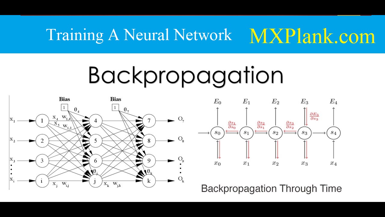
Training a Neural Network with Backpropagation
In the single-layer neural network, the training process is relatively straightforward because the error (or loss function) can be computed as a direct function of the weights, which allows easy gradient computation. In the case of multi-layer networks, the problem is that the loss is a complicated composition function of the weights in earlier layers. The gradient of a composition function is computed using the backpropagation algorithm. The backprop-agation algorithm leverages the chain rule of differential calculus, which computes the error gradients in terms of summations of local-gradient products over the various paths from anode to the output.
Although this summation has an exponential number of components(paths), one can compute it efficiently using
dynamic programming. The backpropagation algorithm is a direct application of dynamic programming.
It contains two main phases, referred to as the
forward and backward phases, respectively.
The forward phase is required to compute the output values and the local derivatives at various nodes,
and the backward phase is required to accumulate the products of these local values over all paths from the
node to the output:
-
Forward phase: In this phase, the inputs for a training instance are fed into the neural network. This results in a forward cascade of computations across the layers, using the current set of weights. The final predicted output can be compared to that of the training instance and the derivative of the loss function with respect to the output is computed. The derivative of this loss now needs to be computed with respect to the weights in all layers in the backwards phase.
-
Backward phase:The main goal of the backward phase is to learn the gradient of the loss function with respect to the different weights by using the chain rule of differential calculus. These gradients are used to update the weights. Since these gradients are learned in the backward direction, starting from the output node, this learning process is referred to as the backward phase.
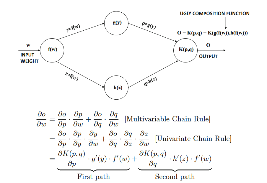
Figure 1.13:Illustration of chain rule in computational graphs:The products of node-specific partial derivatives along paths from weight w to
output o are aggregated. The resulting value yields the derivative of output o with respect to weight w.
Only two paths between input and output exist in this simplified example
Consider a sequence of hidden units
h1,h2,...,hk followed by output
o,
with respect to which the loss function
L is computed.
Furthermore, assume that the weight of the connection from hidden unit
hr to
hr+1 is
w(hr,hr+1).
Then, in the case that a single path exists from
h1 to
o, one can derive the gradient of the loss function
with respect to any of these edge weights using the chain rule:
The aforementioned expression assumes that only a
single path from
h1 to
o exists in the network,
whereas an exponential number of paths might exist in reality. A generalized variant of the chain rule, referred to as the
multivariable chain rule,
computes the gradient in a computational graph, where more than one path might exist. This is achieved by adding the composition along each of the paths
from
h1 to
o .An example of the chain rule in a computational graph with two paths is shown in Figure1.13.
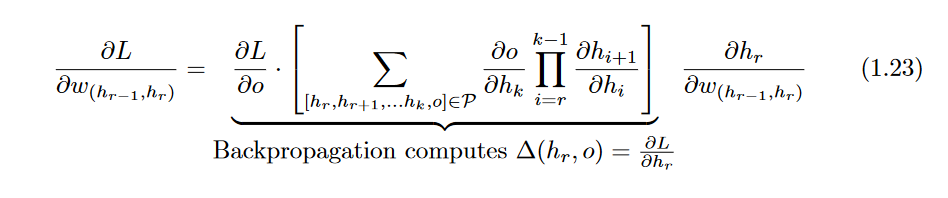
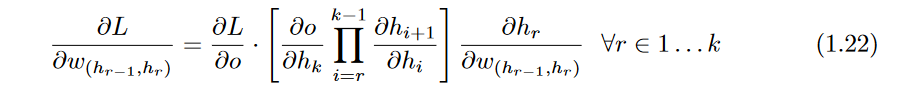
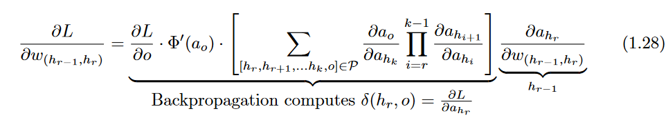
Therefore, one generalizes the above expression to the case where a set
P of paths exist from h
r to
o :
The computation of
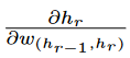
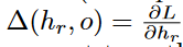
on the right-hand side is straightforward and will be discussed below (see Equation 1.27). However, the path-aggregated term above
[annotated by
Δ(hr,o)= is aggregated over an exponentially increasing number of paths (with respect to path length),
which seems to be intractable at first sight. A key point is that the computational graph of a neural network does not have cycles,and
it is possible to compute such an aggregation in a principled way in the backwards direction by first computing
Δ(hk,o)
for nodes
hk closest to
o, and then recursively computing these values for nodes in earlier layers
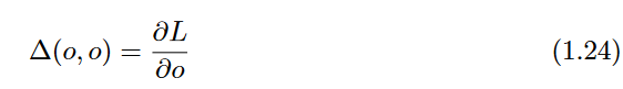
in terms of the nodes in later layers. Furthermore, the value of
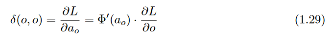
Δ(o, o) for each output node is initialized as follows:
This type of dynamic programming technique is used frequently to efficiently computeall types of path-centric functions
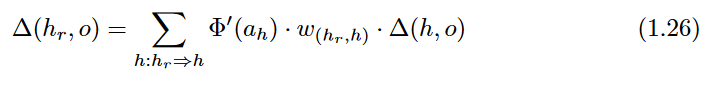
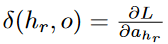
in directed acyclic graphs, which would otherwise require an exponential number of operations. The recursion for
Δ(hr,o)
can be derived using the multi-variable chain rule:
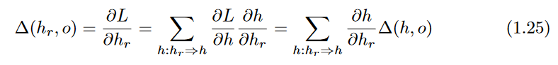
Since each
h is in a later layer than
hr,Δ(h, o) has already been computed while evaluating
Δ(hr,o).
However, we still need to evaluate
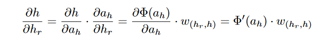
∂h/hr in order to compute Equation1.25.
Consider a situation in which the edge joining
hr to h has weight
w(hr,h), and let
ah be
the value computed in hidden unit h just before applying the activation function Φ(.).
In other words, we have
h=Φ(ah) , where
ah is a linear combination of its inputs from earlier-layer units
incident on
h. Then, by the univariate chain rule, The following expression for
∂h/∂hr can be derived:
This value of
∂h/∂hr is used in Equation1.25, which is repeated recursively in the back-wards direction, starting with the output node. The corresponding updates in the backwards direction are as follows:
Therefore, gradients are successively accumulated in the backwards direction, and each node is processed exactly once in a backwards pass. Note that the computation of Equation 1.25 (which requires proportional operations to the number of outgoing edges ) needs to be repeated for each incoming edge into the node to compute the gradient with respect to all edge weights.
Finally, Equation 1.23 requires the computation of
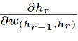
, which is easily computed as follows:
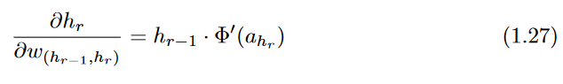
Here, the key gradient that is back-propagated is the derivative with respect to
layer activations, and the gradient with respect to the weights
is easy to compute for any incident edge on the corresponding unit.
It is noteworthy that the dynamic programming recursion of Equation1.26 can be computed in multiple ways,
depending on which variables one uses for intermediate chaining. All these recursions are equivalent in terms of the final result of back propagation.
In thefollowing, we give an alternative version of the dynamic programming recursion, which is more commonly seen in this website.
Note that Equation1.23 uses the variables in the hidden layers as the "chain" variables for the dynamic programming recursion.
One can also use the pre-activation values of the variables for the chain rule. The pre-activation variables in a neuron are obtained after applying
the linear transform (but before applying the activation variables) as the intermediate variables.
The pre-activation value of the hidden variable
h=φ(ah) is ah.
The differences between the pre-activation and post-activation values within a neuron are shown in Figure 1.7 .
Therefore, instead of Equation 1.23 , one can use the following chain rule:
Here, we have introduced the notation
instead of
for setting up the recursive equation. The value of
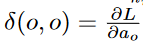
is initialized as follows:
Then, one can use the multivariable chain rule to set up a similar recursion:
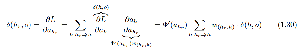
This recursion condition is found more commonly in this website discussing backpropagation.
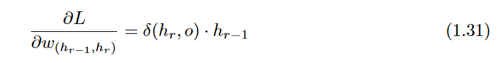
The partial derivative of the loss with respect to the weight is then computed using
∂(hr,o) as follows:
As with the single-layer network, the process of updating the nodes is repeated to convergence by repeatedly cycling through the training data in epochs.
A neural network may sometimes require thousands of epochs through the training data to learn the weights at the different nodes.
A detailed description of the backpropagation algorithm and associated issues will be provided in the coming posts.
In the next post, we will provide a brief discussion of these issues.